How to create 3D charts and XYZ coordinates in Excel
Excel is a spreadsheet application that can render data calculated using 2D charts. The term 2D graph I mean the coordinate system x, y. Visualization of spatial data coordinates x, y, z using a 3D graph does not allow even the latest version (written in 2016). What Excel is presented as a 3D graph is actually only a small cosmetic changes when the data are not shown on the y-axis through moniker but as block certain height, which currently corresponds to the value y. Still, however, this is a graph of x, y (Really 2D).
3D graphs could be used some other software, but it is not easy to link calculations from Excel with some external program. Often it is a problem that I'm not that computer administrator, so you can not install additional programs. On the other hand, Excel is now standard on every computer and even smartphone. In addition to work with Excel can handle any average user. Data visualization in coordinates x, y, z can be done using two simple formulas. This method works well in any other spreadsheet that plots a graph x, y. Even in the old Excel from 1987.
3D objects
 |
Remember how the 3D draws on a paper cube. Draw the square that has all sides equal. Then we draw angled lines directed at an angle of 45 ° at the top right. Their size is not equal to the side of the square, but slightly smaller. We connect the dots loose ends and we got an oblique cube in 3D view. |
What you draw is not a 3D object. It's just a set of lines in a plane substantially only an optical illusion, which reminds us of the 3D cube. To make this a credible illusion, we must follow when drawing according to certain rules. Those we explained in the previous paragraph. To explain this computer, we need rules to describe mathematically. Display (projection) of 3D objects on a 2D plane describes axonometry.
Axonometry - projection onto the plane of the screen
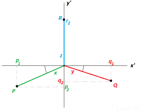
Consider a 3D right-handed coordinate system. In it are placed in 3D space points. Each point in the space of coordinates [x, y, z ]. The 3D space, however, we want to display a 2D computer screen. Like the 3D object casts a shadow on a 2D plane. The image below is a 2D plane of the projection on the screen representation of the coordinates x 'and y'. Us focus on a point P which is reflected from the 3D space to 2D plane x ', y'. Cut down its projection of a 2D x-axis' a particular value of p 1 we know that you calculate using the cosine angle. Similarly, we know calculate the other values P 1, P 2, Q 1, Q 2, r 2nd These numerical values are called coefficients of projection. This could be likened to the fact that when we change the angle of incidence of light and changes the method of projection onto the plane, changing the shape of the shadow.
The transformation equation coefficients and projection
Therefore necessary to specify points in 3D space to the 2D plane of the screen. To serve the general perspective projection transformation equation:
The axis is identical with the axis y, so that the ratio r 1 neglect because r 1 = 0th Coefficients projection need not be calculated manually, because in practice, the most commonly used display already calculated and expressed as the chart values:
| view type | p 1 | p 2 | q 1 | q 2 | r 2 |
| angled left | -0.35 | -0.35 | 1 | 0 | 1 |
| footprint | -1 | 0 | 0 | -1 | 0 |
| draft | -1 | 0 | 0 | 0 | 1 |
| elevation | 0 | 0 | 1 | 0 | 1 |
| angled right | -1 | 0 | 0.35 | -0.35 | 1 |
| General ax. | -0.7 | -0.35 | 0.8 | -0.2 | 0.8 |
We choose, for example, the most widely used type of display called left oblique. Dosadímekonkrétne coefficients in transformation equations. Some expressions in parentheses are multiplied by zero or units, so we get the simplified form:
How to explain to computer
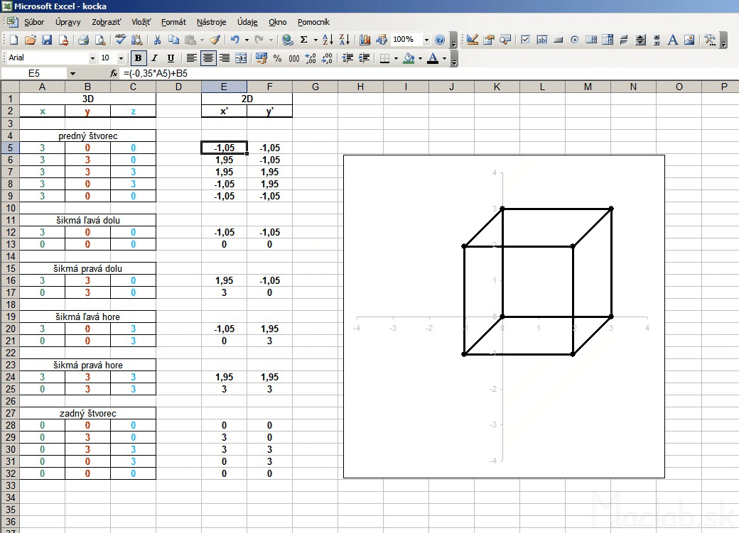
For example, we want to draw dimensional wireframe cube size pages 3 and we want to view it in an oblique view. We start by describe all vertices by coordinates [x, y, z].
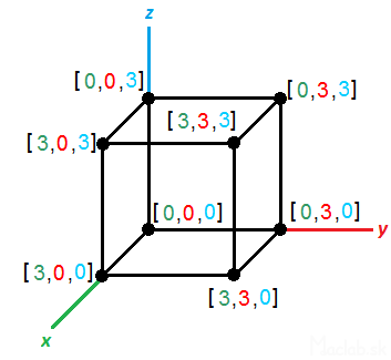
For illustration, I called the coordinates of each color. We create three columns in which they will coordinate points x, y, z describing the position of a point in 3D space. Then, we create two more columns that will be represented in 2D projection of x 'and y'. The first line of columns x 'and y' using the fill patterns for the simplified transformation equations for the x, y, populated with the values of the cells of the first three columns. Coated with the formula to be converted to the full range. Now you just portray the calculated values of the columns x 'and y' using 2D x, y graph. Renders the projection of 3D points to a 2D plane of the screen. The advantage of this solution is that if you change something in 3D coordinates, using the transformation equations are converted 2D projection that is automatically displayed in real time. For better understanding you can download directly sample file kocka.xls .

For a perfect display it needs to have both axis of the graph to scale and that the square area of the graph. Otherwise the image will be flattened. Axis plot the x 'and y' do not need to see and so they can be later removed from the chart, or hide. To draw a line must enter the start and end points. We skip the line and list the points of the other line segments. After selecting the line graph, the segment that will create a projection cubes. Image below is a preview of the file sample kocka-ciary.xls .
Block in 3D space
In another example, we draw the block size with the sides a, b, c. The procedure is similar, but do not enter the coordinates into the columns of x, y, z by hand, but the size ratio of the parallelepiped refer to the shaded cells, which are numerical values of a, b, c. The values of a, b and c can vary, but for convenience I added a dial. Click the arrow up or down to increase or decrease the value in the cell above the dial. These values are populated with up to 3D coordinates, where after transformation into a 2D projection immediately displayed as rendered block.

For Spice up I added even calculate that diverts the vertical edges of the block certain angle. One internal angle block then it is not genuine, but slightly smaller. This will provide monoclinic prism. With the cosine of an angle of deflection, and the calculated new coordinates x, y, z and deployment of new peaks in the area of the prism. You can download the sample file kvader.xls , changing values and track changes.
For a more detailed description of a tutorial can watch a video in which the step by step added to the process illustrated input of coordinates, the downstream projection of the plane x ', y', and the end coordinate calculation according to the ratio of the variable block sizes.
The cylindrical helix
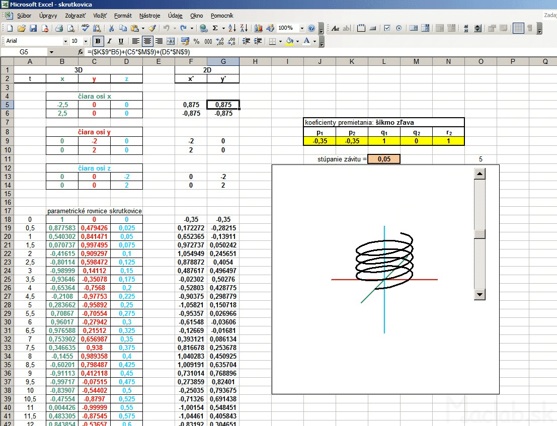
In the following example, I added another column called t. Basically, it's the angle in radians, which is populated with a parametric equation in a cylindrical helix. Parametric equations determine the coordinates x, y, z according to the parameter t. It is a movement along a circular path, and with each revolution (one revolution is 6.28 radians) increases the value of the coordinates to a constant, which is called pitch. Constants can rewrite and use absolute addressing, this constant populated with in each calculation. Thus, we obtain a spatial curve that resembles a spiral.
 |
3D spatial coordinates of the helix needs to be transformed into a 2D projection. Now, however, I use a general transformation equations, with coefficients screening using absolute addressing populated with the yellow fields in the calculations x 'y'. Primetania coefficients P 1, P 2, Q 1, Q 2, R 2 can be rewrite, changing the type of projection and thus display type. The fastest way is to copy the relevant line coefficients from the table directly to the yellow cells in Excel, which can be changed views. Likewise, a change in the 3D coordinates x, y, z in real time converted to 2D and instantly displayed in the graph as projected. Coefficients of projection you can substitute in the masterfile skrutkovica.xls . |
Conical helix
In another example, I created a trio of different projections: general axonometric, side and plan. For each type of projection is the corresponding coefficients are transformed into the coordinates x 'and y'. Of the three columns I had to portray three graphs that show exactly these three views. Coefficients of projection in this example are dosadené to fixed formulas.
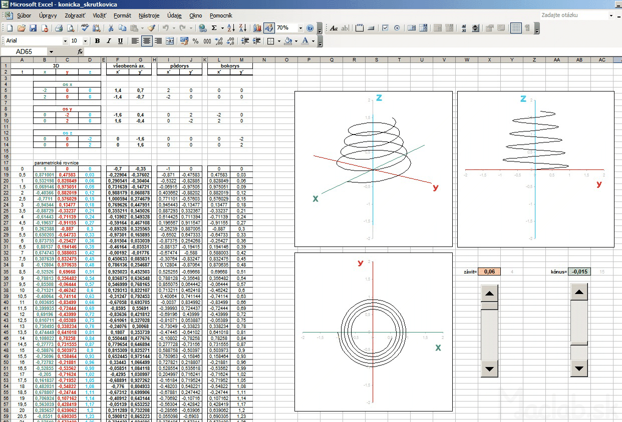
Spice up the formula I has modified the parameter to be changed at each revolution not only the height (pitch) but also the distance from the center. This curve wound is not cylindrical, but conical (cone) surface. The coefficient of taper using sliders and change the value using absolute addressing transferred to the calculation, 3D coordinates. Each change of spatial coordinates after transformation in real time is displayed in three views. This will provide an object that looks like a conical spring. If you do not know exactly how to adjust the general transformation equations for different views, you can download the sample Sobor for this example: pruzina.xls and put all the custom values in column x, y, z.
3D rotation
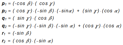
The example on the 3D coordinates are translated into various predefined 2D views using five coefficients projection (taken from the table). In another example, we will show how to make a projection of a view in any arbitrary angle of rotation α, β, γ about axes x, y, z . Now we coefficients projection. considered to be constant, but their numerical values will be recalculated according to the angles α, β, γ . Since the axis ofin 3D space it is not the same as x ' of the 2D space, then neither r1 is not equal to zero, but to another account. And since it is non-zero, we can not neglect. Now therefore we consider it to five, but six of transformation coefficients p 1 , p 2 , q 1 , q 2 , y 1 , y 2 , given by the following formulas:
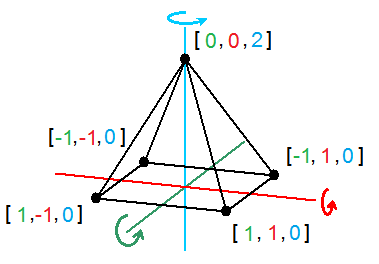
As an example, I created a 3D object pyramid With a footprint the size of 2 and a height of 2, with the center of the base is the same as the center of the 3D coordinate system [ x , y , z ] as the base, and is divided in half 2/2 = 1st
Steering angles α, β, γ is populated with formulas to screening coefficients. Excel must be replaced angles in radians. Since the whole circle has 360 degrees which corresponds to 6.28 radians, then 1 radian is 6.28 / 360 = 0.0174 ° .
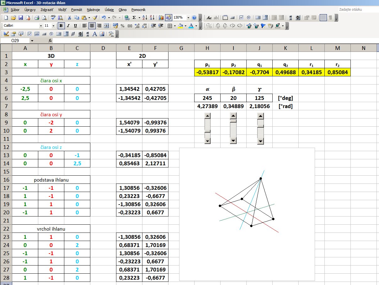
Coefficients calculated projection using absolute addressing populated with transformation equations in the general screening. By varying the angles by using the slider therefore it changes the direction of view from which we look at the 3D object. To illustrate zi Reach sample file: 3D-rotation-ihlan.xls
But it is not rotation in the literal sense, because 3D coordinates do not change, change only the angle of projection on a 2D plane. Rotation of the body in space describe the transformation matrix for rotation. These, however, in this case we do not need, thus considerably simplifying calculations.
A detailed description is in the video below, in which, step by step the process explained by their coordinates, the conversion coefficients of projection according to the angle of the projection onto the plane x ', y'.
GPS
This screening method I used in the display and GPS coordinates. I left a few hours to enable GPS in one place, so I got around 20,000 points in space. The image below is their spatial representation, the tare as cloud points. It is seen that the position determination is always to within a few meters of the center value. More on the evaluation of this experiment can read a separate article on GPS accuracy .
![]()
Other articles:
Calculation of the buildings under the shade