Least squares method
The least squares method is a mathematically statistical method for approximating pairs of measured data [x; y]. By approximation is meant the best possible approach to the real value. The simplest case of using the least squares method is the translation (approximation) of the measured data by the line ŷ = kx + q
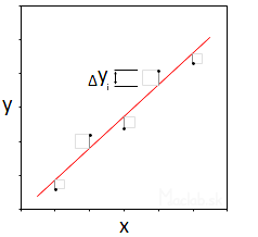 |
We look for the coefficients k and q so that all deviations Δyi are as small as possible. As a criterion, the condition is that the sum of the squares of all deviations must reach a minimum value. We use the square to get a positive value. From a geometric point of view, it is therefore a square.
|
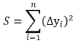
The resulting sum of the areas of all squares must be as small as possible:
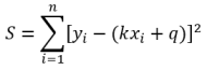
After substituting the functional dependence for the line, the following applies:
We put the partial derivatives of the area according to k and q into equation with zero and solve the equations. The first derivative determines the extreme and the second derivative determines whether it is a maximum or a minimum. However, the maximum in this case is close to infinity.
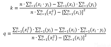
After derivatives and adjustments we get formulas for the coefficients k and q:
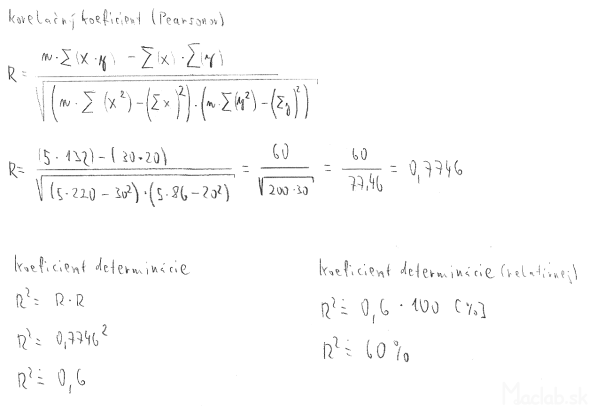
Bravais – Pearson correlation coefficient
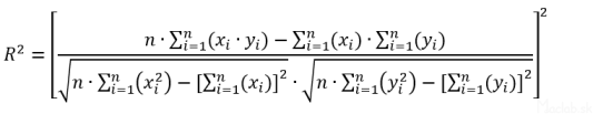
The correlation coefficient (R) expresses the degree of dependence between two variables. Reaches values from -1 to +1. If we exponentiate R, we get values in the range from 0 to 1, which expresses the degree of variance and its value does not depend on the scale of the graph.
The square of the correlation coefficient is called the coefficient of determination (R2). If R2 = 1 then all measured points lie on a straight line, so we have no variance. If R2 = 0 then there is no relationship between the variables. For example, if R2 = 0.81, then 81% of the variability is explained by the linear dependence. The remaining 19% of the variability of the variable y remained unexplained. The value of the coefficient of determination is obtained as the square of the proportion of covariance and the product of variances. After adjustment we get the relationship:
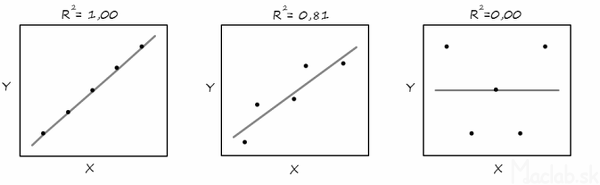
In the figures, the values of R2 for different distributions of point pairs [x; y]
Calculation of optimal line coefficients by least squares method
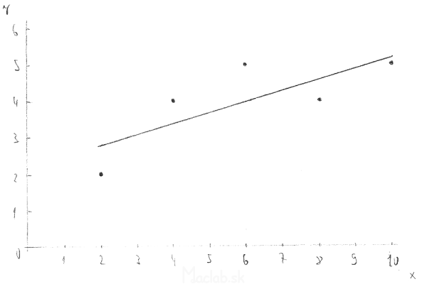
Example: Find a linear function that optimally represents the measured pairs of points [2; 2]; [4; 4]; [6; 5]; [8; 4]; [10; 5]. From the measured points, construct a graph and a curve of the regression function.
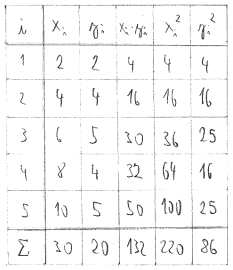 |
We will create a table of measured data. In the formula for calculating the coefficients k and q, certain expressions are often repeated after the symbol sum. We divide these expressions into smaller parts, calculate them into a table and then summarize their values. We have a total of 5 pairs, so the number of all measured pairs [xi; yi] is n = 5.
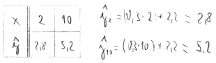
Substitute the summarized values from the table into formulas for calculating the coefficients k and q:
|
Substitute the summarized values from the table into formulas:
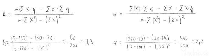
From the coefficients we get the required linear regression function ŷ = 0.3x + 2.2. To draw it, we need to calculate at least two points that belong to it. Usually, the regression curve is plotted at the same interval as the measured data. In our case it is from 2 to 10.
Finally, we draw a graph with measured values and a regression curve into it. We can use several rules to verify the accuracy of the calculations and the graph:
- The average of all xi and yi gives the center of gravity, which lies on the regression curve [6; 4]
- After extending the line, the intersection with the y-axis becomes 2.2
- Arcus tangens 0.3 acquires a value of 16.7 ° which is the angle between the regression curve and the x-axis (in Cartesian coordinates)
Finally, it is necessary to calculate the coefficient of determination, because even with the most accurate measurement we do not achieve 100% accuracy. We will reuse the calculated amounts from the table.
This was the simplest case where the resulting function is a straight line. It is used for linear waveforms and directly proportional quantities. The least squares method can be applied to any curve prescribed by a function. For example hyperbolic, logarithmic, polynomial ...
Related articles: